Introduction

The East African Community is a regional intergovernmental organization comprising eight (8) partner states, namely: Kenya, Tanzania, Uganda, Burundi, Rwanda, South Sudan, Democratic Republic of the Congo, and, most recently, Somalia. Kenya, Tanzania, and Uganda were the founding members in 1967 before the organization dissolved in 1977. The organization was re-established in the year 2000, and new members were accepted in subsequent years: Burundi and Rwanda (2009), South Sudan (2016), Democratic Republic of the Congo (2022), and Somalia (2023).

In this post, I will use ggforce and geom_voronoi_tile() to generate Voronoi diagrams depicting the flags of the East African Community.

This work is inspired by Albert Rapp’s blog post, where he provides examples of the use of ggforce.

Section 1: Load all the required libraries

Code

library(tidyverse)
#install.packages("ggforce")
library(ggforce)
library (patchwork)

Section 2: General equations for generating the voronoi plots

Code

set.seed(23479) # set a random seed for pseudorandom number generator
N <- 1000
voronoi_1 <- tibble(x = runif(N), y = runif(N)) %>% # create a dataset
  ggplot(aes(x, y)) +                               
  geom_voronoi_tile(aes(fill = y))                  # generate the voronoi plot

Section 3: Sample voronoi image

Generated by Albert Rapp

Code

voronoi_1 +
  scale_fill_viridis_c(option = 'A') +
  theme_void() + 
  theme(legend.position = 'none')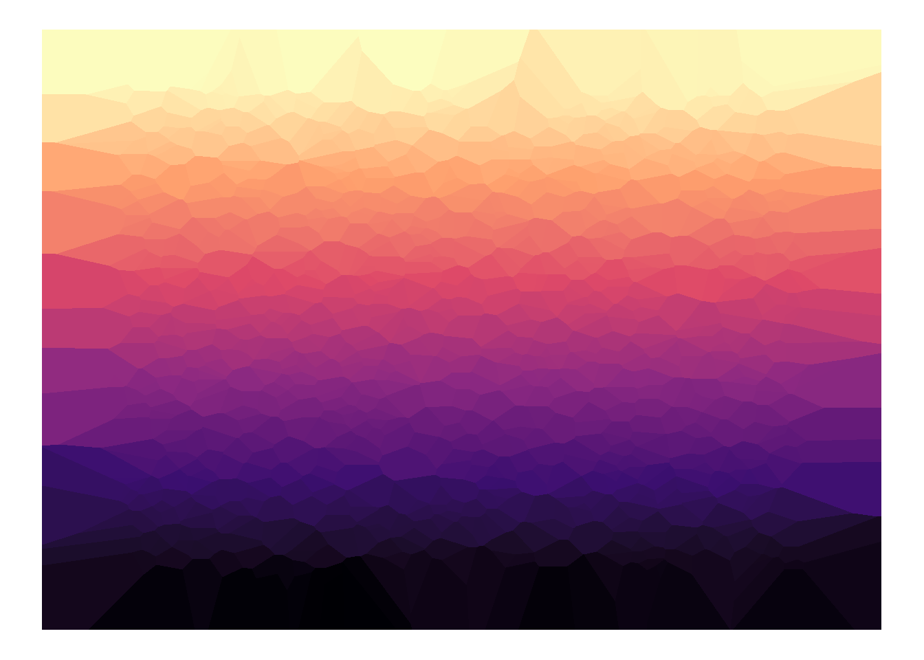

The option in scale_fill_viridis_c() can be set between ‘A’ and ‘H’ and or it can be either “magma”, “inferno”, “plasma”, “viridis”, “cividis”, “rocket”, “mako”, or “turbo.”

The viridis scales provide colour maps that are perceptually uniform in both colour and black-and-white. They are also designed to be perceived by viewers with common forms of colour blindness.

Section 4: Flags of the East African Community and Individual Countries

a) Kenya

Code

ken_1 <- voronoi_1 +
  scale_fill_gradientn(colours = c("#006600", "#FFFFFF", "#BB0000", "#FFFFFF", "#000000")) +
  theme_void() + 
  theme(legend.position = 'none',
        plot.title = element_text(size = 12, hjust = 0.5)) +
  labs(title = "Kenya")
ken_1

b) Tanzania

Code

tan_1 <- voronoi_1 +
  scale_fill_gradientn(colours = c("#00A3DD", "#FBD016", "#000000", "#FBD016","#1EB53A")) +
  theme_void() + 
  theme(legend.position = 'none',
        plot.title = element_text(size = 12, hjust = 0.5)) +
  labs(title = "Tanzania")
tan_1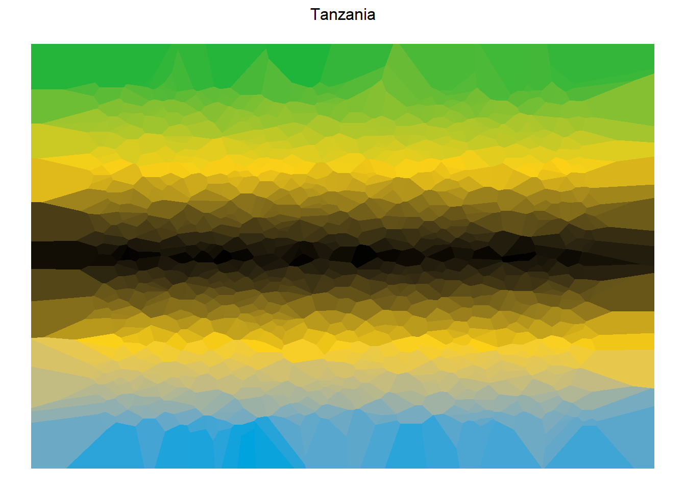

c) Uganda

Code

uga_1 <- voronoi_1 +
  scale_fill_gradientn(colours = c("#D90000", "#FCDC04", "#000000", "#FFFFFF", "#D90000", "#FCDC04", "#000000")) +
  theme_void() + 
  theme(legend.position = 'none',
        plot.title = element_text(size = 12, hjust = 0.5)) +
  labs(title = "Uganda")
uga_1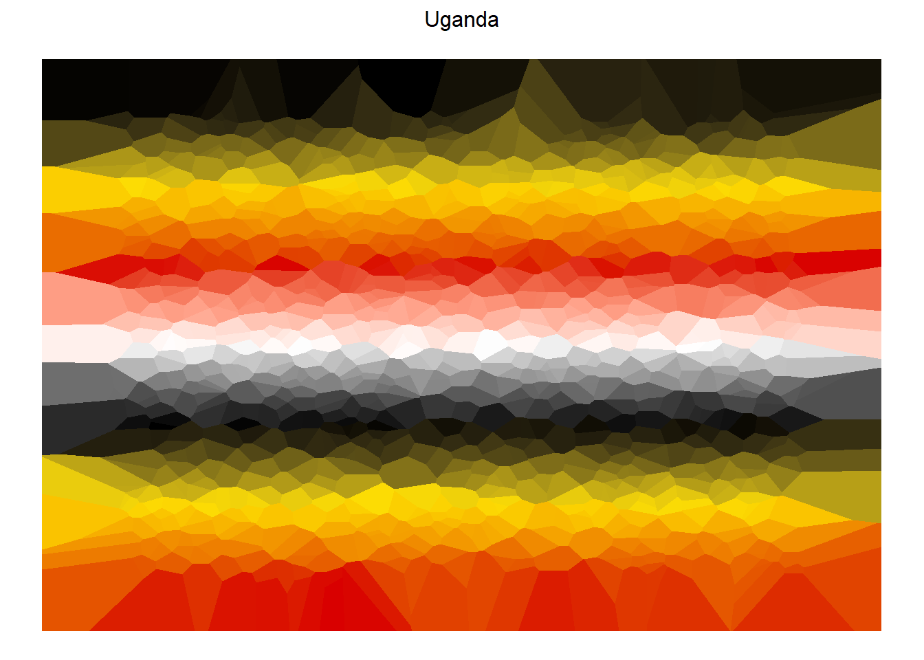

d) Burundi

Code

bur_1 <- voronoi_1 +
  scale_fill_gradientn(colours = c("#CE1126", "#1EB53A", "#FFFFFF", "#1EB53A", "#CE1126")) +
  theme_void() + 
  theme(legend.position = 'none',
        plot.title = element_text(size = 12, hjust = 0.5)) +
  labs(title = "Burundi")
bur_1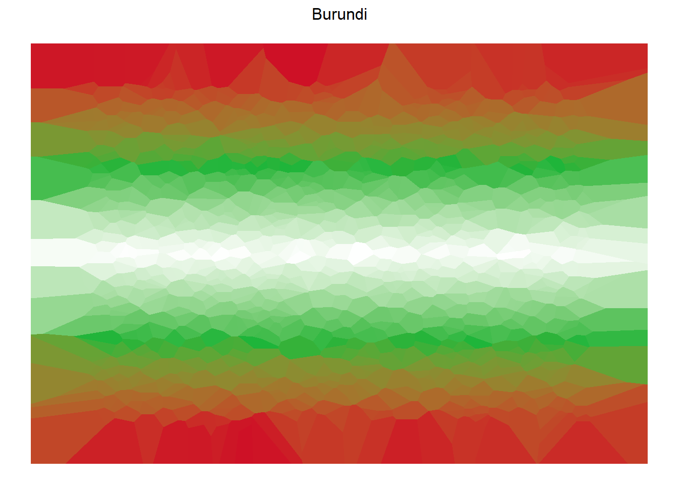

e) Rwanda

Code

rwa_1 <- voronoi_1 +
  scale_fill_gradientn(colours = c("#20603D", "#FAD201", "#00A1DE", "#00A1DE")) +
  theme_void() + 
  theme(legend.position = 'none',
        plot.title = element_text(size = 12, hjust = 0.5)) +
  labs(title = "Rwanda")
rwa_1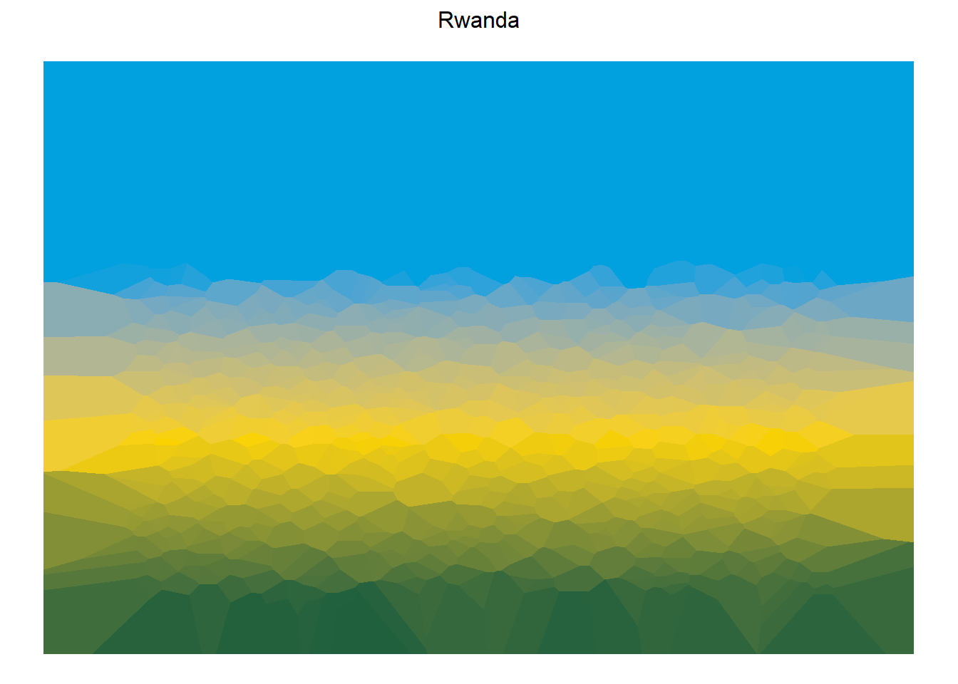

f) South Sudan

Code

ssud_1 <- voronoi_1 +
  scale_fill_gradientn(colours = c("#078930", "#FFFFFF", "#DA121A", "#0F47AF", "#000000")) +
  theme_void() + 
  theme(legend.position = 'none',
        plot.title = element_text(size = 12, hjust = 0.5)) +
  labs(title = "South Sudan")
ssud_1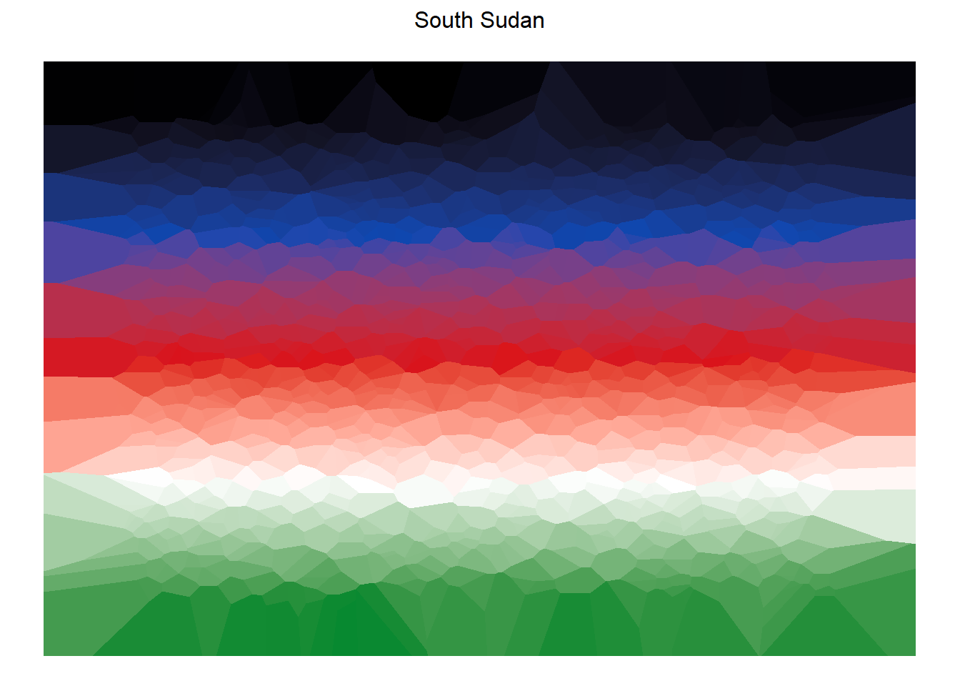

g) Democratic Republic of the Congo

Code

drc_1 <- voronoi_1 +
  scale_fill_gradientn(colours = c("#007FFF", "#F7D518", "#CE1021", "#F7D518", "#007FFF")) +
  theme_void() + 
  theme(legend.position = 'none',
        plot.title = element_text(size = 12, hjust = 0.5)) +
  labs(title = "Democratic Republic of Congo")
drc_1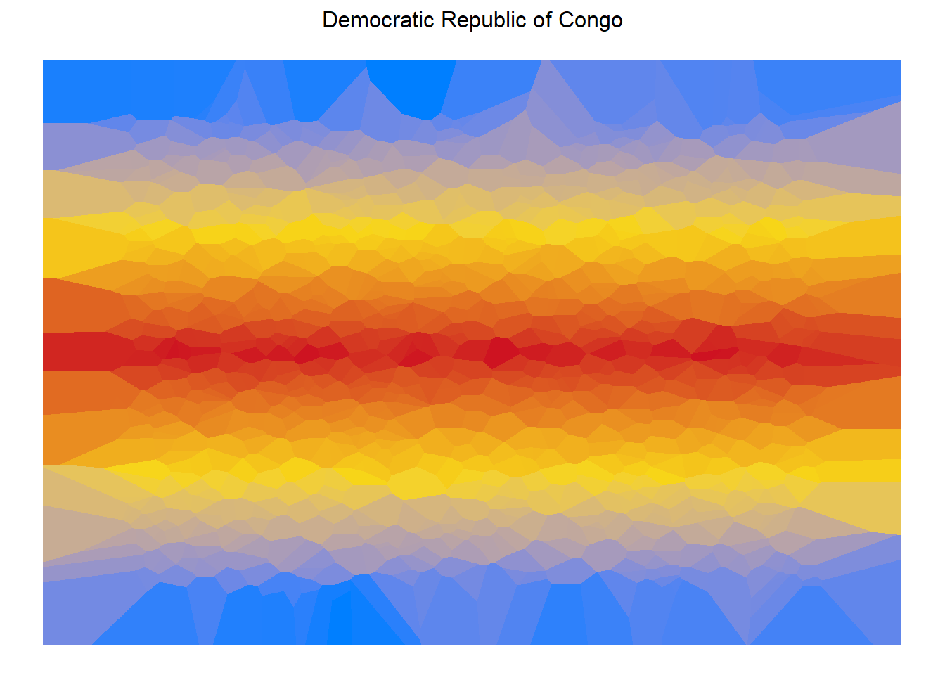

h) Somalia

Code

som_1 <- voronoi_1 +
  scale_fill_gradientn(colours = c("#418FDE", "#FFFFFF", "#418FDE")) +
  theme_void() + 
  theme(legend.position = 'none',
        plot.title = element_text(size = 12, hjust = 0.5)) +
  labs(title = "Somalia")
som_1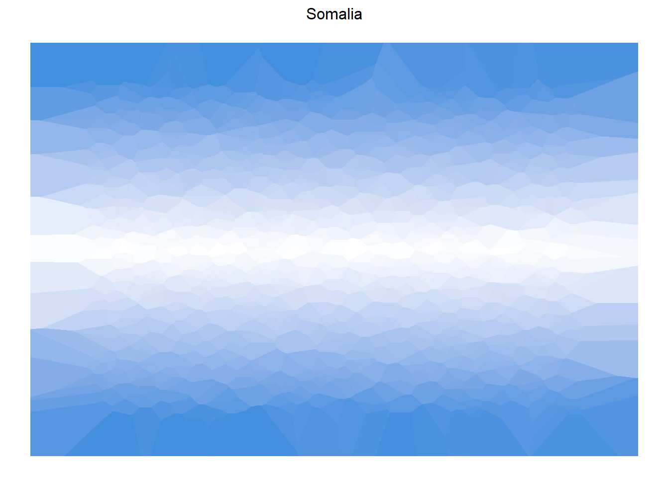

i) East African Community

Code

eac <- voronoi_1 +
  scale_fill_gradientn(colours = c("#418FDE", "#FFFFFF", "#D90000", "#006600","#FBD016", "#006600", "#000000",  "#FFFFFF",  "#418FDE")) +
  theme_void() + 
  theme(legend.position = 'none',
        plot.title = element_text(size = 12, hjust = 0.5)) +
  labs(title = "East African Community")
eac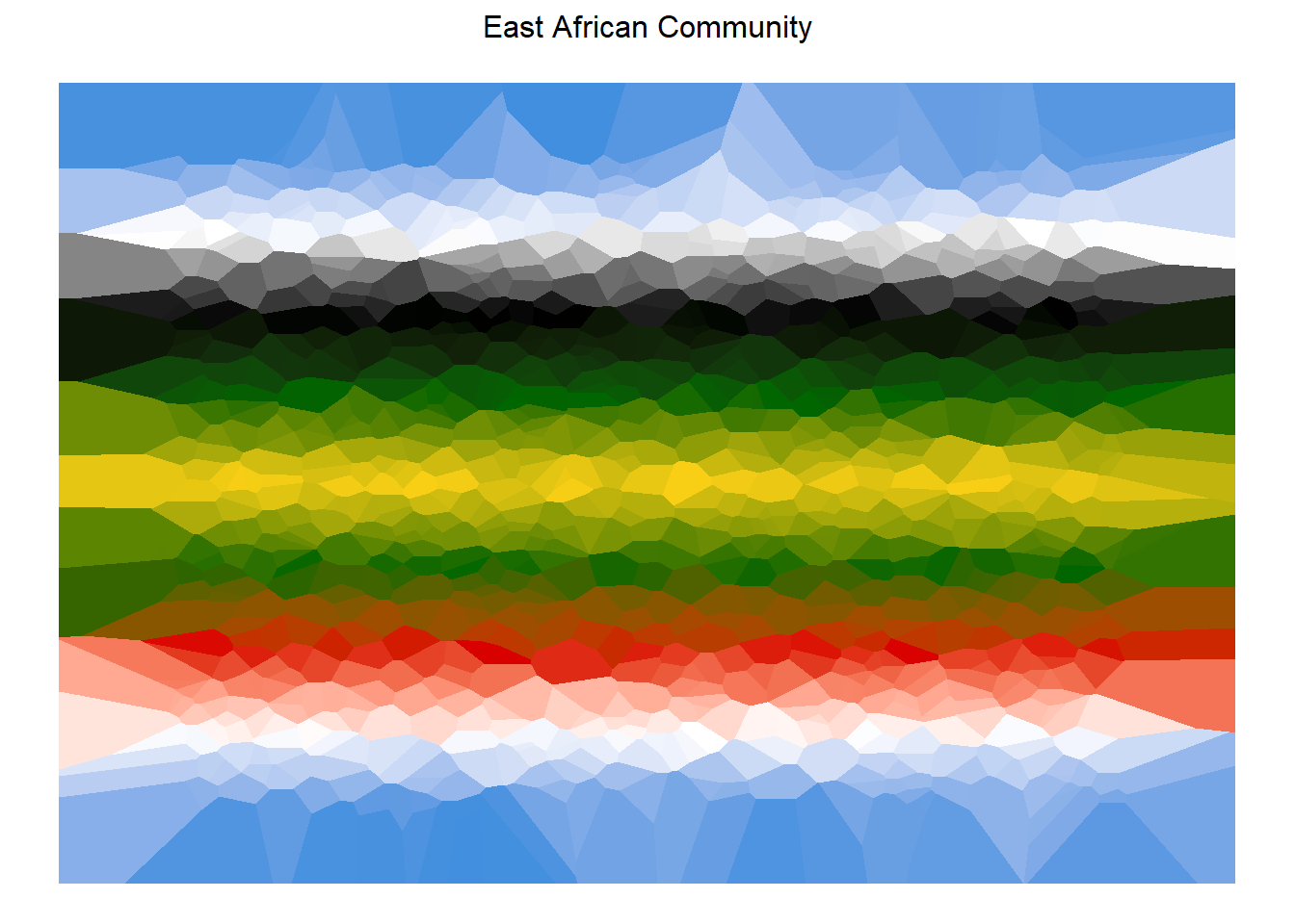

Conclusion

The goal of this post was to demonstrate that one can use code to generate art. Here, the packages, ggplot2 and ggforce, available in R/RStudio, were used to generate Voronoi diagrams (depicting the flags of East Africa) with geom_voronoi_tile(). To compare the generated diagrams with the original flags look at the Flags of the World page on Worldometer

Assignment

Try and generate your own Voronoi diagram (preferably the flag of your home country or country of residence), save with ggsave() using the correct dimensions and dpi, and the share on social media #aRt